Cross-Correlation
This section describes how to perform cross-correlation function (CCF) analysis using the Cross-Correlation Night-Forward module in GUIBRUSHR. The CCF technique detects molecular species in HR spectra by exploiting the Doppler shift of planetary spectral lines due to orbital motion (Brogi et al. 2012, Brogi et al. 2019). The observed data—after telluric removal (Telluric Removal)—are cross-correlated with a template model generated in the Forward Model module (Forward Modeling) across a range of radial velocities.
In this tutorial, we use the equilibrium chemistry model eq_h2o_co containing both H2O and CO to cross-correlate against the IGRINS pre-eclipse observation of WASP-77Ab. The interface is organized into a general configuration panel and two execution panels: one for computing the planetary trail (the CCF as a function of radial velocity and orbital phase), and one for generating the \(K_p\)–\(V_{\mathrm{sys}}\) map that reveals the planetary signal.
General Configuration
The general panel defines the target, model, and dataset to be used:

General configuration panel of the Cross-Correlation Night-Forward module.
Target: select
wasp77Ab.Model CC: the forward model to use as template. Select the model generated in Forward Modeling (
eq_h2o_co).Rad. Transf. Mode: set to
Emissionfor dayside observations.HR Instrument: the spectrograph used for the observations (
igrins).Order Selection: set to
full.Tell rm method: the telluric removal method applied to the data. Must match the method used in Telluric Removal (
PCA_Scikit_Learn).Nights: the available observation nights. Select
20201214.Night sim/syn: leave unchecked for real observations.
UPDATE SELECTION: after selecting the night, click this button to register it. The night appears in the Selection for CC field as
igrins:20201214, confirming that the IGRINS dataset from that date will be used. Multiple nights and/or instruments can be combined by repeating the selection process.
Cross-Correlation – Planetary Trail
The first execution panel computes the cross-correlation between the observed spectra and the template model at each orbital phase, producing the planetary trail map:

Cross-correlation panel for computing the planetary trail. The top row controls the CCF computation, the middle row sets processing options, and the bottom row handles masking.
The panel is organized into three rows:
CCF Parameters (First Row)
CCF filter: if checked, Singular Value Decomposition (SVD) is used to model and subtract the out-of-transit stellar signals from the CCF, effectively isolating the planetary signal by removing systematic noise. Leave unchecked for this tutorial.
Range inf. RV / Range sup. RV: the radial velocity range (in km/s) over which the cross-correlation is computed. Set to
-350and350km/s.Step RV: the velocity step (in km/s) between consecutive cross-correlation evaluations. Set to
1km/s.Phases Bin Size: the bin size for phase averaging. A value of
0.002provides fine sampling of the orbital phase coverage.Type: the weighting scheme for combining CCF values across spectral orders. Select
Weightedto weight each pixel by its error. Normal is associated to classic Person correlation.Ecc. Orbit: to include eccentricity in the trace visualization.
Speed CC: act differently based on the wavelength file. If a single wavelength calibration is associated for all the exposures, the CCF will be faster.
Transit limits: set to
T14to define the transit/eclipse boundaries using the total transit duration (first to fourth contact).
Processing Options (Second Row)
Instrument convolution: when checked, the template model is convolved with the instrumental line profile of the spectrograph before cross-correlation. This should be enabled for accurate results.
Doppler Shadow (DS) correction: if checked, a correction for the Rossiter–McLaughlin effect (Doppler shadow) is applied.
DS width: the width parameter for the Doppler shadow correction (only relevant when the correction is enabled).
maxfev: maximum number of function evaluations for internal optimization routines. The default value of
5000is adequate for most cases.Spectrum selection: set to
Fullto use the complete wavelength range of each spectral order.PDF orders CCF: if checked, diagnostic PDF plots are generated for each individual spectral order’s CCF contribution. Useful for identifying problematic orders, but can be left unchecked to speed up the computation.
CMAP: the colormap used for the trail and CCF plots (
inferno).Extra Kp / Extra rv: trace you to be shown in the plot.
Masking (Third Row)
Mask night: same behavior as the mask for telluric removal.
Mask rv: if checked, enables radial velocity masking to exclude specific velocity ranges from the CCF map (e.g., to remove stellar residuals). When enabled, Min rv mask and Max rv mask define the excluded range in km/s.
Mask phase: if checked, enables orbital phase masking to exclude specific phase ranges. When enabled, Min phase mask and Max phase mask define the excluded range.
For this tutorial, both masks are disabled (set to 0). However, depending on the quality of the telluric removal, users may need to apply a radial velocity mask to exclude stellar residuals that persist after PCA. For instance, masking the range \(-10 < v_{\mathrm{rad}} < 20\) km/s can be effective in removing contamination near the stellar rest frame (see also the reference paper for further details).
Once all parameters are set, click RUN to execute the cross-correlation. The SHOW LAST PLOT button displays the most recently generated trail map.
Cross-Correlation – \(K_p\)–\(V_{\mathrm{sys}}\) Map
The second execution panel generates the \(K_p\)–\(V_{\mathrm{sys}}\) diagram. This map is constructed by co-adding the CCF values along the expected planetary trace for a grid of radial velocity semi-amplitudes (\(K_p\)) and systemic velocities (\(V_{\mathrm{sys}}\)). A significant detection appears as a peak at the expected \(K_p\) and \(V_{\mathrm{sys}}\) of the planet.
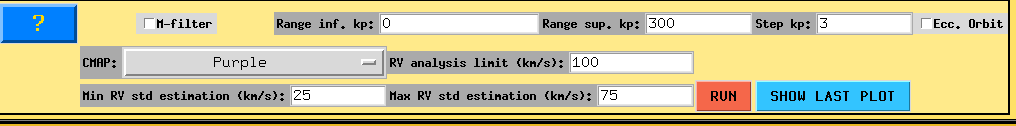
Cross-correlation panel for generating the \(K_p\)–\(V_{\mathrm{sys}}\) map.
M-filter: if checked, a median filter is applied.
Range inf. kp / Range sup. kp: the range of \(K_p\) values (in km/s) to explore. Set to
0and300km/s to cover the expected value of \(K_p \approx 192\) km/s for WASP-77Ab.Step kp: the \(K_p\) step size in km/s. A value of
3provides sufficient sampling to resolve the detection peak.Ecc. Orbit: if checked, an eccentric orbit applied instead of the circular.
CMAP: the colormap for the \(K_p\)–\(V_{\mathrm{sys}}\) diagram. Set to
Purple.RV analysis limit (km/s): the radial velocity range (centered on zero) used for computing the SNR of the detection. Set to
100km/s.Min / Max RV std estimation (km/s): the velocity range used to estimate the noise level (standard deviation) of the CCF map, from which the detection significance (in \(\sigma\)) is derived. Set to
25and75km/s. These values should be chosen to sample a region of the map free from the planetary signal.
Click RUN to generate the \(K_p\)–\(V_{\mathrm{sys}}\) map. The result should show a significant detection peak near the expected values (\(K_p \approx 192\) km/s, \(V_{\mathrm{sys}} \approx 0\) km/s). The SHOW LAST PLOT button allows re-displaying the most recent result.
Users can repeat this analysis with different forward models (e.g., models containing only H2O or only CO) by returning to the general panel and selecting a different Model CC, allowing the investigation of individual molecular contributions to the atmospheric signal.