Forward Modeling
This section describes how to generate a synthetic atmospheric spectrum using the Forward Model module in GUIBRUSHR. The forward model is essential for two purposes: exploring the atmospheric parameter space and producing template spectra for CCF analyses (Cross-Correlation).
In this tutorial, we generate a model in equilibrium chemistry containing both H2O and CO as absorbing species, corresponding to the combined model used for the CCF validation of WASP-77Ab. The atmospheric parameters are set to 10x solar metallicity ([M/H]solar = 1.0) and solar C/O ratio (log(C/O) = -0.26), with an inverted temperature profile. The background atmosphere is composed of H2 and He.
The Forward Model interface is organized into a main configuration panel and a set of subtabs for the detailed atmospheric setup. We describe each component below, following the order in which the user should configure them.
Main Configuration Panel
The top section of the Forward Model module contains the general settings that define the model framework:

Main configuration panel of the Forward Model module, configured for the WASP-77Ab equilibrium chemistry model with H2O and CO.
Target: the planetary system to model (here,
wasp77Ab). Planetary and stellar properties are loaded automatically from the database.Stellar Spectrum: the stellar spectrum used to compute the planet-to-star flux ratio. Options include
Planck(blackbody at the stellar effective temperature) and Phoenix stellar atmosphere models (Husser et al. 2013). For this forward model,Phoenixis selected.Resolution: select
Highfor generating a HR model suitable for CCF analysis with IGRINS data.Rad. Transf. Mode: set to
Emissionfor dayside observations.Chemistry: select
Equilibriumto compute molecular abundances self-consistently from the specified metallicity and C/O ratio via the chemical equilibrium solver (chemcat, Cubillos et al. in prep).T-P profile: select
DoubleIsothermalto use a double isotherm for the temperature–pressure profile.Scattering power law: leave unchecked for this model.
Continuum: set to
H2-H2,H2-Heto include collision-induced absorption from the H2–H2 and H2–He pairs.Include H-: leave unchecked.
Temp Min / Max / Step [K]: these values are not currently used. These are for the future integration of PyratBay (Cubillos et al. 2021).
Radiative transfer code: set to
petitRADTRANS.Min / Max pressure (Eq, 10^): the \(\log_{10}\) pressure boundaries of the atmospheric model, in bar. Set to \(-9\) and \(2\), respectively.
# Pressure Layers: number of atmospheric layers equally spaced in \(\log_{10} P\). Set to
100.LBL Sampling: the line-by-line downsampling factor applied to the native opacity grid (\(R = 10^6\)). A value of
4yields an effective resolution of \(R \sim 2.5 \times 10^5\), sufficient for IGRINS (\(R \approx 45\,000\)).Name model: a user-defined label for this model (here,
eq_h2o_co). This name will be used to identify the model in the database and in subsequent CCF analyses.Min / Max wl HR [\(\mu\) m]: the wavelength range for the model computation. Set to \(0.9\)–\(2.6\;\mu\text{m}\) to cover the full IGRINS spectral range.
Parameters
Note that only the parameters with the checked Present widget will be used in model.
Planet + Data
The Planet + Data subtab contains the fundamental planetary parameters. Most values are automatically loaded from the database when the target is selected:
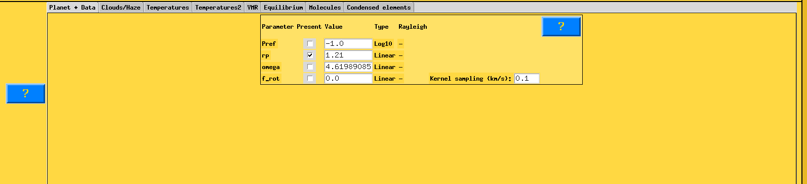
Planet + Data subtab showing planetary parameters for WASP-77Ab.
Pref: the reference pressure level (\(\log_{10}\) bar) at which the planetary radius is defined. Set to \(-1.0\).
rp: the planetary radius in Jupiter radii at the reference pressure level. Set to \(1.21\;R_J\) (Bonomo et al. 2017). The checkbox indicates that this parameter is active. This value defines the baseline atmospheric radius for the radiative transfer calculations.
omega: the planetary rotation rate in d-1 (per day). This parameter controls a convolution kernel that models how solid-body rotation spreads spectral lines in emission or transmission spectroscopy. Set to
4.6199, corresponding to the tidally locked rotation period of WASP-77Ab.f_rot: a rotational scaling factor (in \(\log_{10}\)) associated with the rotational convolution kernel.
Kernel sampling (km/s): the velocity step used for the convolution with the rotational and instrumental line profiles. Set to
0.1km/s.
Clouds/Haze
The Clouds/Haze subtab provides the cloud and haze parameterization. For this tutorial model, clouds are not included; the parameters are shown for reference but are not activated:
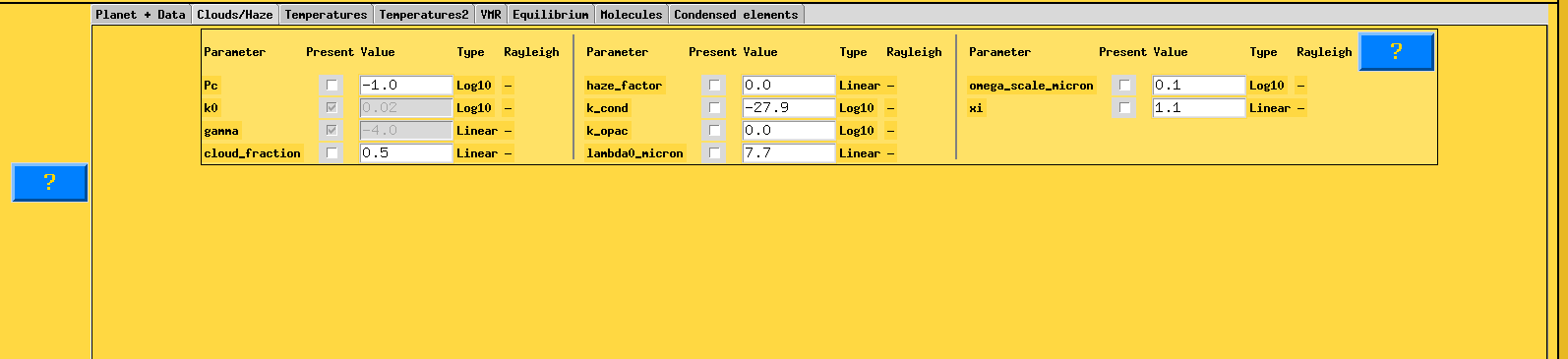
Clouds/Haze subtab. For this tutorial forward model, no cloud parameters are activated.
The available parameters are organized into three groups. The first group controls a power-law opacity model:
Pc: the cloud deck pressure level in \(\log_{10}\) (bar), specifying the pressure depth where the cloud layer forms.
k0: the opacity at the reference wavelength \(\lambda_0 = 0.35\;\mu\text{m}\), in units of cm2/g (\(\log_{10}\)). This sets the normalization of the power-law opacity.
gamma: the power-law index for wavelength-dependent cloud/haze opacity. A value of \(\gamma = -4\) corresponds to Rayleigh-like scattering.
cloud_fraction: combines a clear and a fully cloudy atmosphere as \(F = c_f \times F_{\mathrm{cloudy}} + (1 - c_f) \times F_{\mathrm{clear}}\), where \(c_f\) ranges from 0 (completely clear) to 1 (fully covered).
The second group provides alternative cloud and haze descriptions:
haze_factor: a multiplicative enhancement factor that mimics haze effects by scaling the Rayleigh scattering opacities of the gas.
k_cond: condensate cloud reference opacity in \(\log_{10}\) (cgs units), multiplied by the total atmospheric number density.
k_opac: condensate cloud reference opacity in \(\log_{10}\) (cgs units), representing the product \(k_{\mathrm{cond}} \times n_{\mathrm{tot}}\) directly, following a skewed Gaussian distribution in wavelength.
lambda0_micron: the central wavelength (in \(\mu\text{m}\)) of the Gaussian opacity feature for the condensate model.
The third group controls the shape of the condensate opacity distribution:
omega_scale_micron: the width (\(\log_{10}\), in \(\mu\text{m}\)) of the Gaussian opacity feature in wavelength space.
xi: the skew parameter controlling the asymmetry of the opacity distribution.
For this tutorial, none of these parameters are activated (checkboxes unchecked or parameters in disabled state), as the WASP-77Ab model does not include cloud or haze opacity.
Temperatures
The Temperatures subtab contains the parameters for several pressure–temperature (\(P\)–\(T\)) profile parameterizations available in GUIBRUSHR. Multiple parameterizations coexist in this panel; the active one depends on the T-P profile selection made in the main panel.
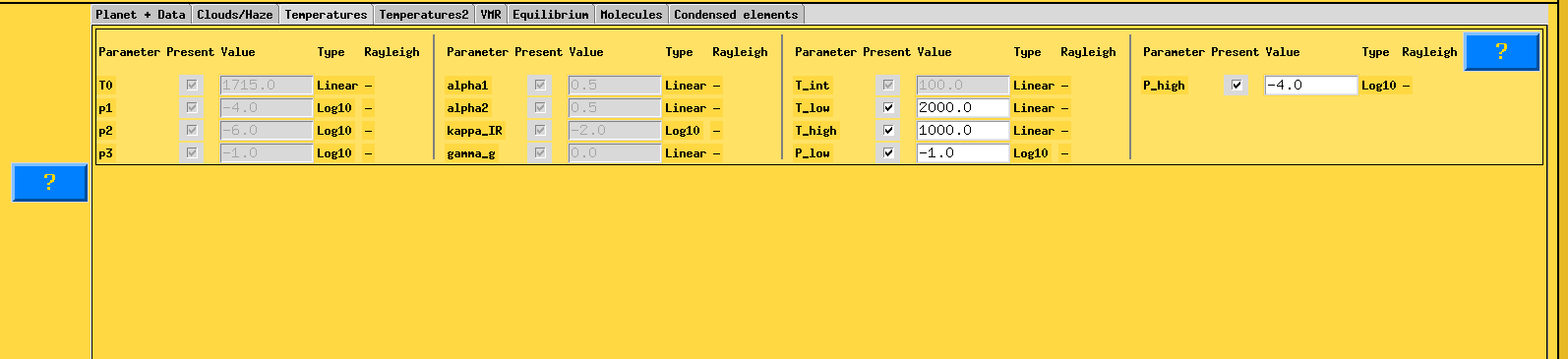
Temperatures subtab showing the available \(P\)–\(T\) profile parameters. The active parameterization depends on the T-P profile selection in the main panel.
The panel displays parameters belonging to different \(P\)–\(T\) profile types:
T0: isothermal atmospheric temperature in Kelvin, used by the
IsothermalandGuillotprofiles.p1, p2, p3: \(\log_{10}\) pressure levels (bar) defining the layer boundaries for the
Madhusudhanprofile.alpha1, alpha2: slopes of the \(T\)–\(P\) relation in the upper and middle layers, respectively (
Madhusudhanprofile).kappa_IR: atmospheric opacity in the IR wavelengths in cm2/g (\(\log_{10}\)), used by the
Guillotprofile.gamma_g: ratio between the optical and IR opacity (
Guillotprofile).T_int: the planetary internal temperature.
Since we selected the DoubleIsothermal profile, the relevant parameters for this model are:
T_low: the lower boundary temperature of the DoubleIsothermal profile. Set to
2000K.T_high: the upper boundary temperature. Set to
1000K.P_low: \(\log_{10}\) pressure of the lower atmospheric boundary (bar). Set to
-1.0.P_high: \(\log_{10}\) pressure of the upper atmospheric boundary (bar). Set to
-4.0.
These values define an inverted temperature profile where the atmosphere is hotter at lower pressures (higher altitudes) in the intermediate layers, consistent with the dayside thermal structure expected for strongly irradiated hot Jupiters. The remaining parameters (T0, p1–p3, alpha1, alpha2, kappa_IR, gamma_g) belong to alternative \(P\)–\(T\) parameterizations and are not used by the DoubleIsothermal profile.
Temperatures2 (Bezier Nodes)
The Temperatures2 subtab is specific to the DoubleIsothermal \(P\)–\(T\) profile and defines the Bezier control nodes (FourNodeSpline) used to construct the temperature profile via spline interpolation (Smith et al. 2024):
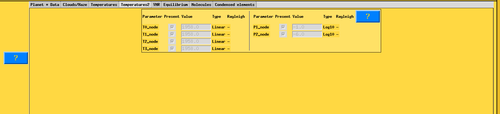
Temperatures2 subtab showing the Bezier node parameterization (FourNodeSpline) for the DoubleIsothermal \(P\)–\(T\) profile.
T0_node: temperature at the first (highest, lowest-pressure) node.
T1_node: temperature at the second node.
T2_node: temperature at the third node.
T3_node: temperature at the fourth (lowest, highest-pressure) node.
P1_node: \(\log_{10}\) pressure (bar) at the second node. The first node is fixed at the top of the atmosphere (\(\log_{10} P = -9\)).
P2_node: \(\log_{10}\) pressure (bar) at the third node. The fourth node is fixed at the bottom of the atmosphere (\(\log_{10} P = 2\)).
VMR
The VMR subtab allows the user to define free-chemistry volume mixing ratio (VMR) profiles for individual molecular species. This tab is used when the Chemistry mode is set to Free; in equilibrium chemistry mode, molecular abundances are computed self-consistently, so this tab remains empty.
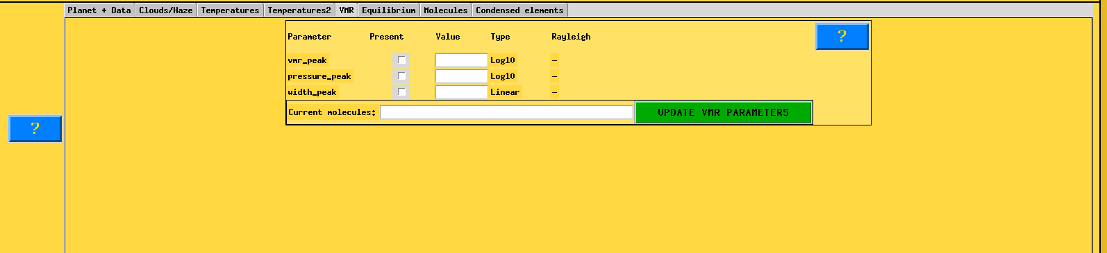
VMR subtab. In equilibrium chemistry mode, this panel is not used; molecular abundances are computed from the metallicity and C/O ratio specified in the Equilibrium tab.
The parameters vmr_peak, pressure_peak, and width_peak allow the definition of a VMR profile that varies with pressure (e.g., a Gaussian-shaped abundance peak). For this tutorial, they are left unchecked.
Equilibrium
The Equilibrium subtab is the key panel for equilibrium chemistry models. It defines the bulk atmospheric composition:
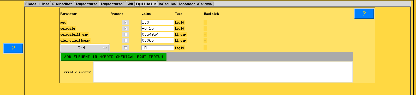
Equilibrium subtab configured with solar metallicity and solar C/O ratio for the WASP-77Ab forward model.
met: the logarithmic atmospheric metallicity [M/H], determining the elemental enrichment relative to hydrogen. A value of
1.0corresponds to 10 x solar metallicity.co_ratio: the carbon-to-oxygen ratio in \(\log_{10}\). A value of
-0.26corresponds to C/O \(\approx 0.55\), i.e., the solar C/O ratio. Also available in the linear format with co_ratio_linear.sio_ratio_linear: the Si/O ratio in linear scale (
0.066, solar value), shown for reference.
The chemical equilibrium solver (chemcat, Cubillos et al. in prep) uses these parameters, together with the \(P\)–\(T\) profile, to compute the self-consistent VMRs of all included molecular species at each atmospheric layer.
The lower part of the panel provides the Hybrid Chemical Equilibrium option, which allows fixing specific elemental abundance ratios (e.g., C/H) while letting the remaining chemistry be computed in equilibrium. This feature is not used in this tutorial.
Molecules
The Molecules subtab defines the atmospheric composition in terms of background gases, continuum absorbers, and molecular species:
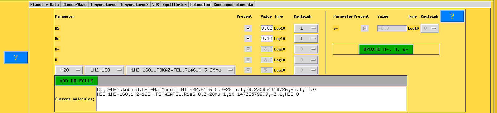
Molecules subtab configured with the background gases (H2, He) and the two absorbing species (CO and H2O) for the equilibrium chemistry forward model.
The upper-left section sets the background gas composition and additional opacity sources:
H2 and He: the bulk VMRs of molecular hydrogen and helium, set to
0.85and0.14(in \(\log_{10}\)), respectively. The Rayleigh column (set to1) activates Rayleigh scattering for these species. These values are used just to define the ratio between the two molecules that will be calculated after defining the metals VMR.H-, H, and e-: additional opacity sources (bound-free and free-free H- absorption, atomic hydrogen, and free electrons). The UPDATE H-, H, e- button recomputes these abundances self-consistently.
The lower section manages the molecular absorbers. To add a molecule, the user selects three items from dropdown menus: the molecule name, its isotopologue, and the specific opacity line list. For this tutorial:
CO: isotopologue
C-O-NatAbund, line listHITEMP.R1e6_0.3-28mu(Rothman et al. 2010).H2O: isotopologue
1H2-16O, line listPOKAZATEL.R1e6_0.3-28mu(Polyansky et al. 2018).
After selecting each molecule, click ADD MOLECULE. The Current molecules field displays all added species with their full configuration strings. In equilibrium chemistry mode, the VMRs of these molecules are computed automatically from the metallicity and C/O ratio; the values shown in the molecule entries (e.g., -5), in this case, is not used. Normally, it serves for the Free Chemistry option.
Condensed Elements
The Condensed elements subtab allows the inclusion of condensate cloud species with microphysical properties. This feature is used for self-consistent cloud modeling with parameters such as the sedimentation factor (cloud_fsed), eddy diffusion coefficient (eddy_diff_coeff), and particle size distribution width (std_radius_distribution).
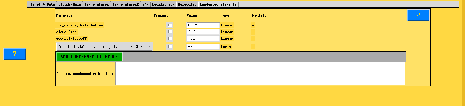
Condensed elements subtab. No condensate species are included in this tutorial forward model.
For this tutorial, no condensed species are added. The panel is shown here for completeness; users working on targets with significant cloud signatures can add condensate species via the ADD CONDENSED MOLECULE button.
Generating the Model
Once all subtabs are configured as described above, return to the main panel and click the execution button (the blue “?” button next to the model name field serves as documentation; the model is generated upon confirmation). The computed spectrum will be stored in the database under the name eq_h2o_co (if saved by pressing the related button) and will be available for selection in the Cross-Correlation module.
Users interested in exploring the parameter space can generate additional models—for instance, a model with only H2O or only CO—by modifying the molecular species in the Molecules tab and saving under a different model name.